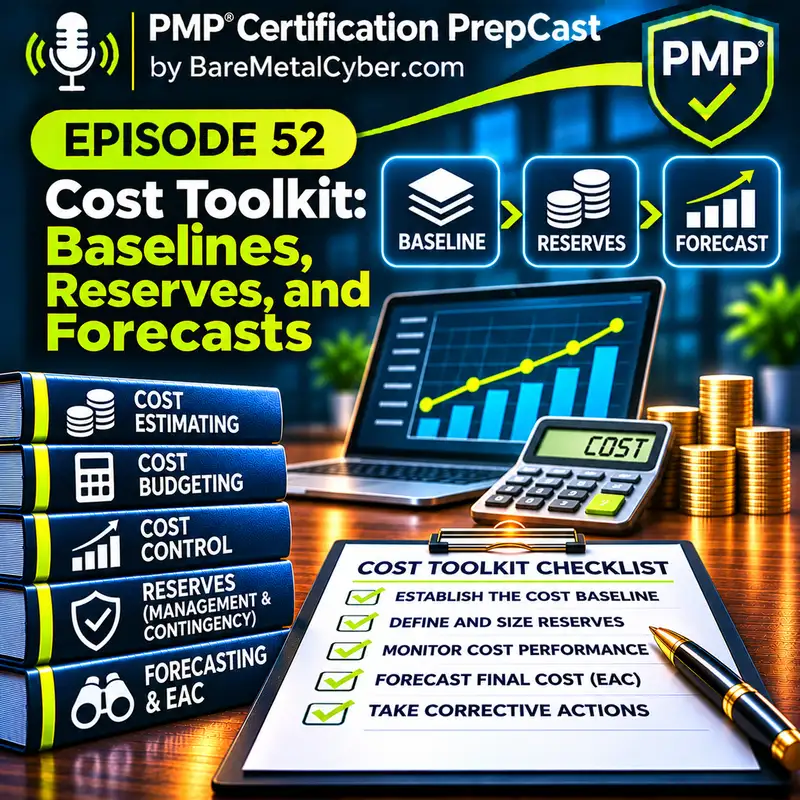
PMP 2026 | 52 | Cost Toolkit: Baselines, Reserves, and Forecasts
Cost management provides the discipline needed to plan, control, and explain project costs transparently. This toolkit connects estimating, budgeting, actual costs, commitments, reserves, and credible forecasts. It applies to predictive, adaptive, and hybrid work without requiring every project to use the same funding model. Early visibility matters because a cost problem, a cash timing problem, and a lack of spending authority may require different decisions. A useful report makes those distinctions clear before a missed payment or exhausted reserve forces the issue.
Welcome to Certified, the P M P prepcast. This is episode fifty two of season one. Today we are exploring cost baselines, reserves, and forecasts based on earned value and remaining work.
Defendable budgets require more than numbers, they require traceability and rationale. Stakeholders must understand how estimates were developed, what reserves were included, and how funding will be distributed over time. When budgets can be explained transparently, confidence grows, and approvals are easier to secure. Realistic forecasts help teams adjust early rather than facing surprises at the end. Early detection of variance, supported by earned value management or agile burn rates, allows corrective action while there is still time to recover. P M I emphasizes that project managers act as stewards of resources, not just recordkeepers. On the exam, correct answers emphasize traceability, reserves, and integration across baselines.
Cost management applies across delivery approaches. A predictive plan may time-phase cost by work package, while a stable iterative team may forecast part of its cost from the expected number of iterations. Include other project costs and make the assumptions explicit. Iterative completion is not the same as realized benefit, and agile work can still operate under a formal budget and approval limits. Match measurement and reporting to the actual funding and delivery decisions.
Building a cost baseline begins with estimating costs. Estimates may draw on historical data, vendor quotes, or parametric models that link costs to key drivers such as labor hours or material quantities. Once estimates are developed, contingency reserves are added. These reserves cover known-unknowns, identified risks and uncertainty addressed through the project’s reserve planning. For example, if a supplier delay is a recognized risk, contingency dollars are set aside to cover overtime or expedited shipping. Management reserves are then considered separately. These cover unknown-unknowns and sit outside the baseline, controlled by the designated management authority. On the exam, stems about “mixing reserves” test this distinction. Correct answers emphasize contingency inside, management outside.
The baseline is not just a single number; it is a time-phased view of spending. Costs must be aligned to the schedule so that funding is available when expenses are incurred. This prevents gaps where teams are ready to work but money has not been allocated. Funding limits must be defined, and spending curves, often called S-curves, help visualize when expenditures peak and taper. P M I emphasizes that time-phased budgets allow integration with earned value management, where performance is measured against both cost and schedule. On the exam, distractors that suggest “baseline as lump sum” are incomplete. Correct answers emphasize phased costs tied to schedule.
Resourcing and procurement decisions also drive the cost baseline. Labor rates, staff capacity, and utilization assumptions must be documented. Materials, equipment, and software licenses often represent major line items that must be timed with project milestones. Vendor pricing and contract terms introduce further complexity, especially when exchange rates or escalation clauses are involved. Make-or-buy analysis determines whether work should be performed internally or outsourced, and contract type influences risk sharing. For example, fixed-price contracts transfer risk to the seller, while cost-reimbursable contracts leave more exposure with the buyer. On the exam, stems about “ignoring contract implications” highlight weak planning.
Approval thresholds and escalation paths must be clear. Not every expenditure or variance requires escalation to a steering committee. Small deviations may fall within delegated authority, while larger ones require formal approval. By publishing thresholds, the project manager avoids delays from unnecessary escalations and protects governance from being overwhelmed. Similarly, procurement policies often define approval levels for vendor commitments. Integrating these thresholds into the cost plan ensures that decisions can be made quickly but remain compliant. On the exam, distractors that suggest “every variance goes to governance” are inefficient. Correct answers emphasize thresholds and defined escalation paths.
Capture actual costs accurately and use the same reporting cutoff as the work-performance data. Accruals recognize costs incurred before payment, while outstanding commitments identify future exposure under purchase orders or contracts. Reconcile these categories so the same obligation is not counted twice as both an actual cost and an outstanding commitment. The cost baseline, total project budget, remaining commitment, cash available, and authority to spend answer different questions. A project can look healthy against its budget while still facing a near-term funding shortage. Clear reporting makes those differences visible before an invoice or delivery forces a rushed decision.
Variance reporting keeps stakeholders informed. Instead of flooding them with raw data, the project manager provides reports at a steady cadence, highlighting exceptions. For example, a report may state, “We are within budget overall, but vendor costs are running ten percent higher than forecast.” Exception-based reporting reduces noise while maintaining trust. Linking spend to delivered value and risk reduction also strengthens credibility. Stakeholders are more willing to support additional funding when they see tangible benefits. On the exam, distractors that suggest “more detail equals better reporting” are incomplete. Correct answers emphasize cadence, exceptions, and value linkage.
Linking cost reports to delivered value creates meaning. For instance, reporting that five hundred thousand dollars has been spent is less helpful than explaining that the spend delivered three completed features that enable early revenue. Similarly, explaining that contingency spend reduced a risk exposure strengthens justification. By framing cost in terms of outcomes, project managers shift the conversation from “what did we spend?” to “what did we gain?” P M I stresses that this value-centric lens builds trust and protects benefits realization. On the exam, distractors that present costs in isolation are traps. Correct answers emphasize connecting dollars to outcomes and risk reduction.
A proposed cost change needs an impact assessment proportionate to its consequences. Adding staff may accelerate a suitable activity but increase cost; reducing scope may save money while weakening benefits or breaching an agreement. Check the delegated authority, applicable thresholds, and any already approved response. Seek further approval when the proposed action crosses those limits. Immediate protective action may already be authorized, and a current forecast should not be withheld while a funding decision is pending.
Keep the approved baseline and the current forecast separate. Update a forecast as soon as credible evidence changes the expected outcome, even when no baseline change has been approved. Show the variance against the existing approved baseline so stakeholders can see the problem. A baseline changes only through its authorized control process; it must not be rewritten merely to hide unfavorable performance. Once a change is approved, record the new baseline and its rationale while retaining the history. Honest forecasting supplies the evidence needed for approval rather than waiting for approval to acknowledge reality.
Communication is the final piece of cost change control. Every approved change must be communicated with rationale to stakeholders, explaining what was decided, why it was necessary, and how it affects benefits. This closes the loop and prevents rumors or confusion. Documentation must be updated so that artifacts reflect the decision, not just verbal agreements. P M I emphasizes that cost management is as much about communication as calculation. On the exam, distractors that suggest “implement silently” highlight poor governance. Correct answers emphasize documenting and communicating decisions visibly.
Earned value management compares the budgeted value of planned and completed work with its actual cost. Planned value is the authorized budget assigned to work scheduled by the data date. Earned value is the budget assigned to work actually completed under the agreed measurement rule. Actual cost is the cost incurred for that work, not merely invoices paid. Schedule variance equals earned value minus planned value and is expressed in the same budget units, not days. Cost variance equals earned value minus actual cost. Earned value describes budgeted work accomplishment; it does not measure revenue, user benefit, or the business value ultimately realized.
The schedule performance index is earned value divided by planned value, when planned value is positive. One means the project has earned the amount of budgeted work planned by that data date; a value below one signals less budgeted work accomplished than planned. It does not, by itself, establish the finish date or prove that a critical milestone is late. The cost performance index is earned value divided by actual cost, when actual cost is positive. A value below one means the completed work cost more than its budgeted value. Use these measures alongside schedule logic and the reasons for the variance.
An estimate at completion depends on an explicit assumption about the remaining work. If the observed cost efficiency is expected to continue, one estimate divides the budget at completion by the cost performance index. If the remaining work is expected to follow its original budget, add actual cost to the budget at completion minus earned value. If both cost and schedule performance are expected to affect the cost of the remaining work, add actual cost to the remaining budgeted work divided by the product of the cost performance index and schedule performance index. The entire remaining-work amount belongs above that product in the fraction. Where conditions have changed materially, a fresh bottom-up estimate of remaining work may be more credible than extrapolating a ratio.
From E A C, you can calculate the Estimate to Complete, abbreviated E T C. This is simply the estimate at completion minus the actual cost already spent. It represents the forecasted cost of the remaining work. Another useful measure is the To-Complete Performance Index, or T C P I. This shows the cost efficiency needed to complete the project within a certain target, either the original budget at completion or the new estimate at completion. It is calculated by dividing the remaining work, budget minus earned value, by the remaining funds, either budget minus actual cost or estimate at completion minus actual cost. Calculate only when the denominator is positive, and compare the required future efficiency with credible delivery conditions. The ratio indicates how demanding a target is; it does not prove the target is achievable.
Choose the measure that answers the decision in front of you. If earned value data are available, cost and schedule indexes help identify patterns, but they do not establish a cause or dictate one forecast formula. A low cost index may reflect recurring inefficiency or an unusual cost that will not recur. A schedule index needs network and milestone context before you infer a cost consequence. State why the remaining work should behave like the historical work, or why it should behave differently, and use a bottom-up forecast when the old assumptions no longer hold.
Consider a fictional distribution-center upgrade with a cost baseline of six hundred thousand dollars. That baseline includes sixty thousand dollars of contingency. A separate sixty thousand dollars of management reserve brings the total project budget to six hundred sixty thousand dollars. At a common status date, planned value is three hundred thousand dollars, earned value is two hundred forty thousand dollars, and actual cost is three hundred thousand dollars. Those values describe the same authorized work and use the agreed progress-credit and cost-recognition rules.
The cost variance is earned value minus actual cost, giving negative sixty thousand dollars. The schedule variance is earned value minus planned value, also negative sixty thousand dollars. These equal numbers have different meanings. The cost variance compares accomplishment with its incurred cost. The schedule variance compares accomplishment with the budgeted work scheduled by this date. Neither calculation says the project is sixty days late, and neither measures the operational benefit of the new center.
Dividing earned value by actual cost produces a cost performance index of zero point eight. Dividing earned value by planned value also produces a schedule performance index of zero point eight. The identical ratios should not tempt you to combine the explanations. A project can accomplish substantial inexpensive work off the critical path while a costly critical activity waits. To forecast the delivery date, examine the schedule network and remaining durations. To forecast cost, ask which efficiency assumptions plausibly apply to the remaining work.
If the current cost efficiency continues, six hundred thousand divided by zero point eight gives an estimate at completion of seven hundred fifty thousand dollars. This is a conditional forecast, not a discovered final invoice. It assumes the future cost of completing the authorized work will behave like the observed cost efficiency. If the poor performance came from a one-time setup expense and the remaining work can follow its original budget, add actual cost of three hundred thousand to remaining budgeted work of three hundred sixty thousand. That different assumption gives six hundred sixty thousand dollars.
The team instead develops a fresh remaining-work estimate. Outstanding supplier commitments, excluding everything already incurred, total one hundred eighty thousand dollars. Internal labor, testing, and other remaining uncommitted costs total two hundred ten thousand dollars. Together these form a remaining estimate of three hundred ninety thousand dollars. Added to actual cost of three hundred thousand, the bottom-up forecast becomes six hundred ninety thousand dollars. Validate what is included in those categories rather than adding every available financial total together.
Suppose someone adds the entire original purchase order to actual cost and the new remaining estimate. Part of that purchase order has already been delivered and recognized as an actual cost, so the calculation counts the same obligation twice. Reconcile the order into incurred amounts, remaining binding commitments, and any cancellable or optional elements. A purchase order total is useful for contractual control, but it is not automatically an extra amount on top of every other forecast category. Ask finance and procurement to confirm a mutually exclusive breakdown.
Under the bottom-up forecast, estimate to complete is three hundred ninety thousand dollars. Variance at completion is the six hundred thousand dollar baseline minus the six hundred ninety thousand dollar forecast, giving negative ninety thousand dollars. The forecast is also thirty thousand dollars above the total project budget, even before debating which reserves may be used. A manager who reports only that there is sixty thousand dollars of management reserve has not explained the remaining shortfall or established that using that reserve is appropriate.
The sponsor asks whether the team can still finish at the original six hundred thousand dollar baseline. The to-complete performance index compares remaining budgeted work of three hundred sixty thousand dollars with remaining funds of three hundred thousand dollars. The required ratio is one point two, compared with the observed zero point eight. That is a substantial change in required future efficiency. The calculation does not forbid recovery, but it creates a precise question: what credible changes in work methods, costs, or conditions would support that target?
Using six hundred ninety thousand as a proposed target produces a different denominator. The remaining amount is three hundred ninety thousand dollars, so the required future efficiency is approximately zero point nine two three. This is less demanding than one point two but still above the observed efficiency. A fresh estimate may support it because the remaining work differs from completed work. Explain those differences. Selecting a new target in a calculation does not authorize extra funding, alter scope, or convert the forecast into an approved baseline.
Now separate cash from cost. Finance has released three hundred sixty thousand dollars. Payments made total two hundred sixty thousand dollars, while a further forty thousand dollars has been incurred but not yet paid. Actual cost is therefore three hundred thousand under the agreed recognition basis. Cash remaining from the current release is one hundred thousand dollars. If one hundred forty thousand dollars is due before the next planned release, including the accrued amount, there is a forty thousand dollar timing gap. Paying later would not erase an incurred cost, and an approved total budget would not automatically remove the timing constraint.
The financial decision now has several distinct parts. Finance can investigate whether a permitted funding release can be advanced. The project team can validate the remaining-work forecast and identify feasible efficiencies. The designated approval body can evaluate any additional funding or scope change. These activities may proceed together, but their authorities are not interchangeable. The project manager should not promise a supplier money that has not been made available or suppress the forecast while waiting for the preferred funding answer.
Reserve use requires its own classification. Suppose an identified transport risk occurs and the approved response requires ten thousand dollars from allocated contingency. The risk becoming an issue does not invalidate that planned response. Record the trigger, confirm the delegated spending authority, and track the draw against the reserve already inside the baseline. If a different unforeseen in-scope condition requires twenty thousand dollars of management reserve, request it from the designated owner. An approved transfer into the baseline could increase that baseline while leaving the total authorized project budget unchanged.
A new request for an additional loading area is different again. It changes the deliverable boundary and needs its scope and funding decision; calling it unforeseen does not make it an automatic management-reserve expense. These distinctions help the sponsor see whether the problem is performance, uncertainty, new scope, cash timing, or several at once. Close the review with the current forecast, the assumptions behind it, the next payment constraint, and the specific decisions required. Numbers become useful when each one answers a clearly named question.
Some adaptive projects fund a stable cross-functional team for an iteration and forecast a range of total team cost from the expected number of iterations. Include other relevant costs, such as supplier work, licenses, facilities, and transition support. Team funding and velocity are optional planning choices, not universal agile requirements. Completed features are outputs; benefits such as reduced waiting or increased adoption require their own evidence. Hybrid projects can report these costs against a project baseline while retaining the assumptions and uncertainty behind each forecast.
Throughput, cycle time, and velocity answer different questions. Throughput counts completed items per defined time period. Cycle time measures elapsed time for an item between agreed workflow boundaries. Velocity totals completed estimation units per iteration. If a team costs twenty thousand dollars for an iteration and completes ten comparable items, the average team cost is two thousand dollars per item: cost divided by item count. It is not cost multiplied by throughput. Changes in work size, quality, or other costs can make that average misleading, so use it with context and keep benefit measures separate.
Let’s consider a scenario. A project shows a cost performance index less than one, meaning costs are higher than expected, while the schedule performance index is about one, meaning budgeted work accomplishment is roughly at the planned level. The milestone forecast still needs schedule analysis. The sponsor asks whether the team should cut scope or add people. The best next action is not to leap to drastic moves but to analyze variance drivers. Perhaps quality rework is inflating costs, or perhaps vendor pricing increased unexpectedly. The project manager proposes targeted corrective action, such as resequencing value slices or addressing specific quality processes, rather than broad cuts. The estimate at completion is updated and options are communicated.
This scenario highlights the importance of interpretation over raw numbers. A C P I less than one does not automatically mean scope should be cut or staff increased. It means each dollar of actual cost has earned less budgeted work value than planned; that is different from measuring business benefit. Only by analyzing the cause can corrective action be targeted effectively. Scope cuts may undermine benefits, while adding people may accelerate schedule but further increase cost. P M I emphasizes that earned value metrics must be explained, not just calculated. On the exam, distractors that suggest immediate scope cuts or staffing changes are traps. Correct answers emphasize variance analysis before action.
Common pitfalls in cost management include re-baselining too early, mixing reserves, and performing math without interpretation. Re-baselining first hides problems rather than solving them, undermining trust. Mixing contingency and management reserves creates confusion about who controls funds and when they can be used. Performing E V M math without explaining meaning leaves stakeholders with numbers but no insight. Other pitfalls include hiding committed spend, which causes budget shocks, and overreacting to normal variance noise without looking for trends. On the exam, distractors often embody these errors. Correct answers emphasize governance discipline, reserve clarity, and meaningful interpretation of metrics.
Another pitfall is ignoring vendor exposure. Projects often commit funds through purchase orders or contracts long before invoices arrive. If these commitments are not tracked, the project may appear under budget until large bills come due. P M I stresses that committed spend is part of cost reality and must be visible in reports. Overreacting to noise is another error. A single bad week may not mean a trend. Project managers must differentiate between normal fluctuations and systemic problems. On the exam, correct answers emphasize tracking commitments and looking for patterns, not reacting to isolated data points.
Plan a time-phased cost baseline with appropriate contingency and distinguish management reserve. Reconcile actual costs, accruals, and outstanding commitments. Interpret performance measures using consistent cutoffs, then forecast with assumptions suited to the remaining work. Address urgent obligations and use delegated authority when available; obtain additional approval where required. Keep the current forecast separate from approved baseline changes and connect spending to intended outcomes without claiming every cost immediately produces a realized benefit.
The cost toolkit is strongest when its categories remain distinct and connected. Budget describes an authorized limit, a baseline supports performance measurement, a forecast describes the expected outcome, and funding describes availability over time. Combine those views with clear scope, reserve ownership, and cost-recognition rules. Then communicate the evidence and the required decision, preserving both the history of performance and the authority to change commitments.
For more certification study resources, books, and podcasts, visit Bare Metal Cyber dot com. Thank you for listening to Certified, the P M P prepcast.